3.4: Graphs of Polynomial Functions

We have already explored the local behavior (the location of $x$- and $y$-intercepts) for quadratics, a special case of polynomials. In this section we will explore the local behavior of polynomials in general.

Identify Zeros and Their Multiplicities from a Graph

Graphs behave differently at various $x$-intercepts. Sometimes, the graph will cross over the horizontal axis at an intercept. Other times, the graph will touch the horizontal axis and bounce off. Suppose, for example, we graph the function

$Graph of f(x)=(x+3)(x-2)^2(x+1)^3.$

Notice in the figure to the right illustrates that the behavior of this function at each of the $x$-intercepts is different.

The $x$-intercept −3 is the solution of equation $(x+3)=0$. The graph passes directly through the $x$-intercept at $x=−3$. The factor is linear (has a degree of 1), so the behavior near the intercept is like that of a line—it passes directly through the intercept. We call this a single zero because the zero corresponds to a single factor of the function.

The $x$-intercept 2 is the repeated solution of equation $(x−2)^2=0$. The graph touches the axis at the intercept and changes direction. The factor is quadratic (degree 2), so the behavior near the intercept is like that of a quadratic—it bounces off of the horizontal axis at the intercept. The factor is repeated, that is, $(x−2)^2=(x−2)(x−2)$, so the solution, $x=2$, appears twice. The number of times a given factor appears in the factored form of the equation of a polynomial is called the multiplicity. The zero associated with this factor, $x=2$, has multiplicity 2 because the factor $(x−2)$ occurs twice.

The $x$-intercept −1 is the repeated solution of factor $(x+1)^3=0$. The graph passes through the axis at the intercept, but flattens out a bit first. This factor is cubic (degree 3), so the behavior near the intercept is like that of a cubic—with the same S-shape near the intercept as the toolkit function $f(x)=x^3$. We call this a triple zero, or a zero with multiplicity 3.

Graphical Behavior of Polynomials at $x$-intercepts

If a polynomial contains a factor of the form $(x−h)^p$, the behavior near the $x$-intercept is determined by the power $p$. We say that $x=h$ is a zero of multiplicity $p$.

The graph of a polynomial function will touch the $x$-axis at zeros with even multiplicities.
The graph will cross the $x$-axis at zeros with odd multiplicities.
The higher the multiplicity, the flatter the curve is at the zero.
The sum of the multiplicities is the degree of the polynomial function.

For zeros with even multiplicities, the graphs touch or are tangent to the $x$-axis. For zeros with odd multiplicities, the graphs cross or intersect the $x$-axis. See the figure below for examples of graphs of polynomial functions with a zero of multiplicity 1, 2, and 3. The graphs clearly show that the higher the multiplicity, the flatter the graph is at the zero.

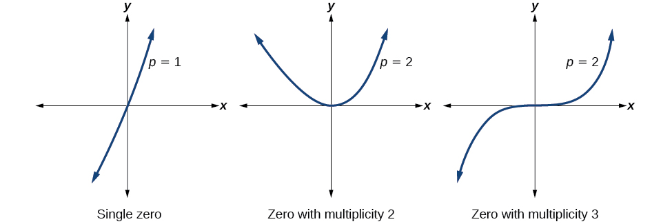
$Three graphs showing three different polynomial functions with multiplicity 1, 2, and 3.$

For higher even powers, such as 4, 6, and 8, the graph will still touch and bounce off of the horizontal axis but, for each increasing even power, the graph will appear flatter as it approaches and leaves the $x$-axis. For higher odd powers, such as 5, 7, and 9, the graph will still cross through the horizontal axis, but for each increasing odd power, the graph will appear flatter as it approaches and leaves the $x$-axis.

How to: Given a graph of a polynomial function, identify the zeros and their mulitplicities

If the graph crosses the $x$-axis at a zero, it is a zero with odd multiplicity.
If the graph touches and bounces off of the $x$-axis, it is a zero with even multiplicity.
The higher the multiplicity of the zero, the flatter the graph gets at the zero.

Example $\PageIndex$: Find Zeros and Their Multiplicities From a Graph

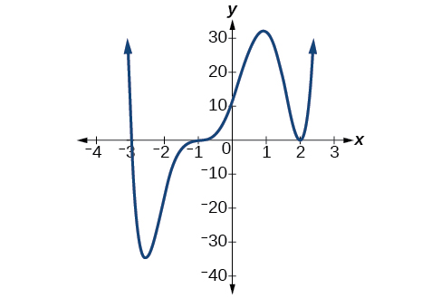
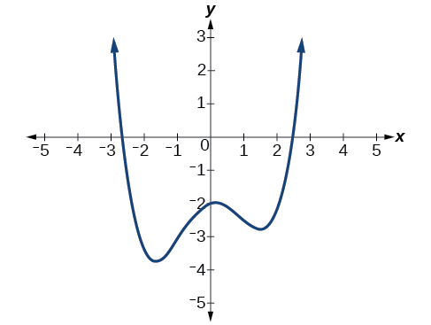
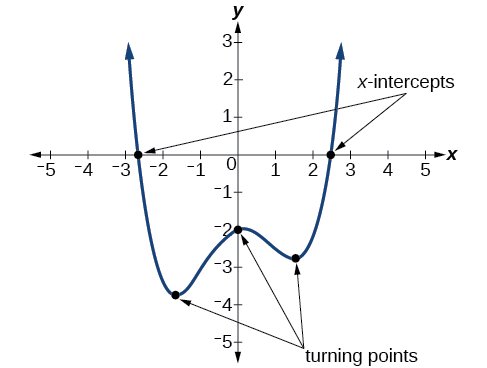
Use the graph of the function of degree 6 in the figure below to identify the zeros of the function and their possible multiplicities.

Solution

Starting from the left, the first zero occurs at $x=−3$. The graph touches the $x$-axis, so the multiplicity of the zero must be even. The zero of −3 has multiplicity 2.

The next zero occurs at $x=−1$. The graph looks almost linear at this point. This is a single zero of multiplicity 1.

The last zero occurs at $x=4$. The graph crosses the $x$-axis, so the multiplicity of the zero must be odd. Since the graph is flat around this zero, the multiplicity is likely 3 (rather than 1).

The polynomial function is of degree $6$ so the sum of the multiplicities must be at least $2+1+3$ or $6$.

Try It $\PageIndex$

Use the graph of the function in the figure below to identify the zeros of the function and their possible multiplicities.

$Graph of a polynomial function with degree 5.$

Graph of a polynomial function.

Answer

The zero at -5 is odd. Since the curve is somewhat flat at -5, the zero likely has a multiplicity of 3 rather than 1.
The zero at -1 has even multiplicity of 2.
The zero at 3 has even multiplicity. Since the curve is flatter at 3 than at -1, the zero more likely has a multiplicity of 4 rather than 2.

Find Zeros and their Multiplicities from a Polynomial Equation

Recall that if $f$ is a polynomial function, the values of $x$ for which $f(x)=0$ are called zeros of $f$. If the equation of the polynomial function can be factored, we can set each factor equal to zero and solve for the zeros.

How to: Given an equation of a polynomial function, identify the zeros and their multiplicities

Factor the polynomial as a product of linear factors (of the form $(ax+b)$), and irreducible quadratic factors (of the form $(ax^2+bx+c).$ When irreducible quadratic factors are set to zero and solved for $x$, imaginary solutions are produced. Write each repeated factor in exponential form.
If the exponent on a linear factor is even, its corresponding zero has even multiplicity equal to the value of the exponent and the graph will touch the $x$-axis and turn around at this zero.
If the exponent on a linear factor is odd, its corresponding zero has odd multiplicity equal to the value of the exponent, and the graph will cross the $x$-axis at this zero.
The sum of the multiplicities plus the number of imaginary zeros is equal to the degree of the polynomial.

Example $\PageIndex$: Find zeros and their multiplicity from a factored polynomial

Find the zeros and their multiplicity for the following polynomial functions.

Solution.

a) This polynomial is already in factored form. All factors are linear factors.

Starting from the left, the first factor is $x$, so a zero occurs at $x=0 $. The exponent on this factor is $1$ which is an odd number. Therefore the zero of $ 0$ has odd multiplicity of $1$, and the graph will cross the $x$-axis at this zero.
The next factor is $(x+1)^2$, so a zero occurs at $x=-1 $. The exponent on this factor is $ 2$ which is an even number. Therefore the zero of $-1$ has even multiplicity of $2$, and the graph will touch and turn around at this zero.
The last factor is $(x+2)^3$, so a zero occurs at $x= -2$. The exponent on this factor is $ 3$ which is an odd number. Therefore the zero of $-2 $ has odd multiplicity of $3$, and the graph will cross the $x$-axis at this zero.

b) This polynomial is partly factored. All the zeros can be found by setting each factor to zero and solving

The factor $x^2= x \cdot x$ which when set to zero produces two identical solutions, $x= 0$ and $x= 0$
The factor $(x^2-3x)= x(x-3)$ when set to zero produces two solutions, $x= 0$ and $x= 3$
The factor $(x^2+4)$ when set to zero produces two imaginary solutions, $x= 2i$ and $x= -2i$. Since these solutions are imaginary, this factor is said to be an irreducible quadratic factor.
The factor $(x^2-x-6) = (x-3)(x+2)$ when set to zero produces two solutions, $x= 3$ and $x= -2$
The factor $(x^2-7)$ when set to zero produces two irrational solutions, $x= \pm \sqrt$

Now we need to count the number of occurrences of each zero thereby determining the multiplicity of each real number zero.

The solution $x= 0$ occurs $3$ times so the zero of $0$ has multiplicity $3$ or odd multiplicity.
The solution $x= 3$ occurs $2$ times so the zero of $3$ has multiplicity $2$ or even multiplicity.
The real number solutions $x= -2$, $x= \sqrt$ and $x= -\sqrt$ each occur $1$ time so these zeros have multiplicity $1$ or odd multiplicity.
The imaginary solutions $x= 2i$ and $x= -2i$ each occur $1$ time so these zeros have multiplicity $1$ or odd multiplicity but since these are imaginary numbers, they are not $x$-intercepts.

Try It $\PageIndex$

Find the zeros and their multiplicity for the polynomial $f(x)=x^4-x^3−x^2+x$.

Answer

Zeros $-1$ and $0$ have odd multiplicity of $1$. Zero $1$ has even multiplicity of $2$

Graph Polynomial Functions

We can use what we have learned about multiplicities, end behavior, and intercepts to sketch graphs of polynomial functions. Let us put this all together and look at the steps required to graph polynomial functions.

How to: Given a polynomial function, sketch the graph

Determine the end behavior by examining the leading term.
Find the intercepts and use the multiplicities of the zeros to determine the behavior of the polynomial at the $x$-intercepts.
Use the end behavior and the behavior at the intercepts to sketch a graph.
Optionally .
- Check for symmetry. If the function is an even function, its graph is symmetrical about the $y$-axis, that is, $f(−x)=f(x)$. If a function is an odd function, its graph is symmetrical about the origin, that is, $f(−x)=−f(x)$.
- Ensure that the number of turning points does not exceed one less than the degree of the polynomial.
- Use technology to check the graph.

Example $\PageIndex$: Sketch the Graph of a Polynomial Function

Sketch a graph of $f(x)=−2(x+3)^2(x−5)$.

Solution

Step 1. The leading term, if this polynomial were multiplied out, would be $−2x^3$, so the end behavior is that of a vertically reflected cubic, with the the graph falling to the right and going in the opposite direction (up) on the left: $ \nwarrow \dots \searrow $ See Figure $\PageIndex$.

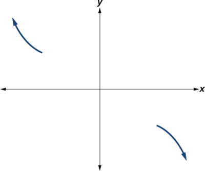
$Showing the distribution for the leading term.$

Figure $\PageIndex$: Illustration of the end behaviour of the polynomial.

This graph has two $x$-intercepts. At $x=−3$, the factor is squared, indicating a multiplicity of 2. The graph will bounce at this $x$-intercept. At $x=5$, the function has a multiplicity of one, indicating the graph will cross through the axis at this intercept.

The $y$-intercept is found by evaluating $f(0)$.

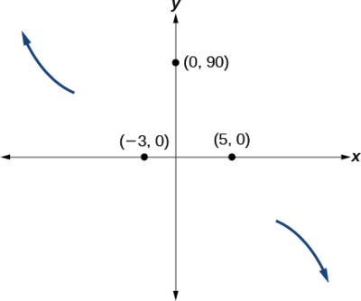
$Graph of the end behavior and intercepts, (-3, 0), (0, 90) and (5, 0), for the function f(x)=-2(x+3)^2(x-5).$

Figure $\PageIndex$: The graph crosses at $x$-intercept $(5, 0)$ and bounces at $(-3, 0)$. The $y$-intercept is $(0, 90)$.

Step 3. Connect the end behaviour lines with the intercepts.

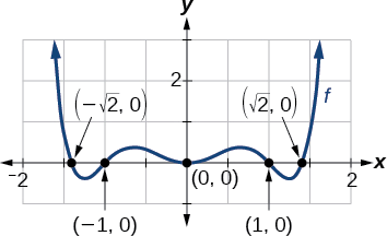
Sketch a graph of $f(x)=x^2(x^2−1)(x^2−2)$. State the end behaviour, the $y$-intercept, and $x$-intercepts and their multiplicity.

Solution

Step 1. The leading term is the product of the high order terms of each factor: $ (x^2)(x^2)(x^2) = x^6$.
The leading term is positive so the curve rises on the right.
The degree of the leading term is even, so both ends of the graph go in the same direction (up). $\qquad \nwarrow \dots \nearrow $

Step 2. The $y$-intercept can be found by evaluating $f(0)$. So $f(0)=0^2(0^2-1)(0^2-2)=(0)(-1)(-2)=0 $.

The $x$-intercepts can be found by solving $f(x)=0$. Set each factor equal to zero.

This gives us five $x$-intercepts: $ (0,0)$, $(1,0)$, $(−1,0)$, $(\sqrt,0)$, and $(−\sqrt,0)$.
The $x$-intercepts $(1,0)$, $(−1,0)$, $(\sqrt,0)$, and $(−\sqrt,0)$ all have odd multiplicity of 1, so the graph will cross the $x$-axis at those intercepts.
The $x$-intercept $(0,0)$ has even multiplicity of 2, so the graph will stay on the same side of the $x$-axis at 2. (The graph is said to be tangent to the x- axis at 2 or to "bounce" off the $x$-axis at 2).

Step 3. The polynomial is an even function because $f(-x)=f(x)$, so the graph is symmetric about the y-axis. The graph appears below.

$An even function$

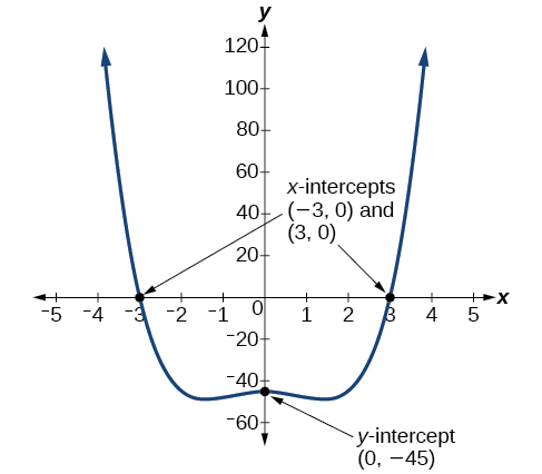
Sketch a graph of the polynomial function $f(x)=x^4−4x^2−45$. State the end behaviour, the $y$-intercept, and $x$-intercepts and their multiplicity.

Solution

Step 1. The leading term is $x^4$.
The leading term is positive so the curve rises on the right.
The degree of the leading term is even, so both ends of the graph go in the same direction (up). $\qquad \nwarrow \dots \nearrow $

Step 2. The $y$-intercept occurs when the input is zero.

The $y$-intercept is $(0,−45)$.

The $x$-intercepts occur when the output is zero. To determine when the output is zero, we will need to factor the polynomial.

The $x$-intercepts $(3,0)$ and $(–3,0)$ all have odd multiplicity of 1, so the graph will cross the $x$-axis at those intercepts.

Step 3. The polynomial is an even function because $f(-x)=f(x)$, so the graph is symmetric about the y-axis. The graph appears below. The imaginary zeros are not $x$-intercepts, but the graph below shows they do contribute to "wiggles" (truning points) in the graph of the function.

$Graph of f(x)=x^4-4x^2-45, which labels all the intercepts at (-3, 0), (3, 0), and (0, -45).$

Try It $\PageIndex$

Sketch a graph of $f(x)=\dfrac(x−1)^3(x+3)(x+2)$.

$CNX_PreCalc_Figure_03_04_215.jpg$

Answer

Turning Points

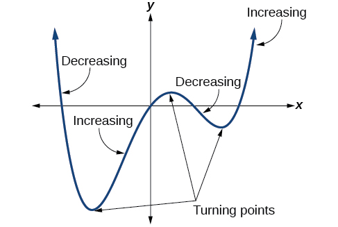
Definition: Turning Points

A turning point is a point of the graph where the graph changes from increasing to decreasing (rising to falling) or decreasing to increasing (falling to rising).

A polynomial of degree $n$ will have, at most, $n$ $x$-intercepts and $n−1$ turning points.

The degree of a polynomial function helps us to determine the number of $x$-intercepts and the number of turning points. A polynomial function of $n$ th degree is the product of $n$ factors, so it will have at most $n$ roots or zeros. When the zeros are real numbers, they appear on the graph as $x$-intercepts. The graph of the polynomial function of degree $n$ can have at most $n–1$ turning points. This means the graph has at most one fewer turning points than the degree of the polynomial or one fewer than the number of factors.

$Graph of f(x)=x^4-x^3-4x^2+4x which denotes where the function increases and decreases and its turning points.$

The maximum number of turning points of a polynomial function is always one less than the degree of the function.

Example $\PageIndex$: Find the Maximum Number of Turning Points of a Polynomial Function

Find the maximum number of turning points of each polynomial function.

$f(x)=−x^3+4x^5−3x^2+1$
$f(x)=−(x−1)^2(1+2x^2)$

Solution

First, rewrite the polynomial function in descending order: $f(x)=4x^5−x^3−3x^2+1$

Identify the degree of the polynomial function. This polynomial function is of degree 5.

The maximum number of turning points is $5−1=4$.

First, identify the leading term of the polynomial function if the function were expanded: multiply the leading terms in each factor together.

Then, identify the degree of the polynomial function. This polynomial function is of degree 4.

The maximum number of turning points is $4−1=3$.

Example $\PageIndex$: Find the Maximum Number of Intercepts and Turning Points of a Polynomial

Without graphing the function, determine the maximum number of $x$-intercepts and turning points for $f(x)=−3x^+4x^7−x^4+2x^3$.

Solution

The polynomial has a degree of $n$=10, so there are at most 10 $x$-intercepts and at most 9 turning points.

Try It $\PageIndex$

Without graphing the function, determine the maximum number of $x$-intercepts and turning points for $f(x)=108−13x^9−8x^4+14x^+2x^3$

Answer

There are at most 12 $x$-intercepts and at most 11 turning points.

Example $\PageIndex$: Drawing Conclusions about a Polynomial Function from the Factors

Given the function $f(x)=−4x(x+3)(x−4)$, determine the $y$-intercept and the number, location and multiplicity of $x$-intercepts, and the maximum number of turning points.

Solution

The $y$-intercept is found by evaluating $f(0)$.

The $y$-intercept is $(0,0)$.

The $x$-intercepts are found by determining the zeros of the function.

The three $x$-intercepts $(0,0)$,$(–3,0)$, and $(4,0)$ all have odd multiplicity of 1.

The degree is 3 so the graph has at most 2 turning points.

Try It $\PageIndex$

Given the function $f(x)=0.2(x−2)(x+1)(x−5)$, determine the local behavior.

Answer

The function is a 3rd degree polynomial with three $x$-intercepts $(2,0)$, $(−1,0)$, and $(5,0)$ all have multiplicity of 1, the $y$-intercept is $(0,2)$, and the graph has at most 2 turning points.

Example $\PageIndex$: Drawing Conclusions about a Polynomial Function from the Graph

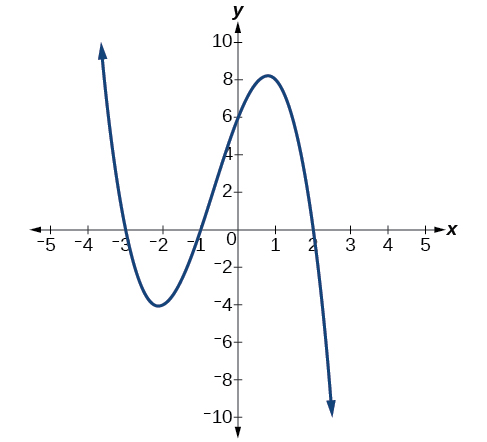
What can we conclude about the degree of the polynomial and the leading coefficient represented by the graph shown below based on its intercepts and turning points?

$Graph of an even-degree polynomial.$

Solution

$Graph of an even-degree polynomial that denotes the turning points and intercepts.$

The end behavior of the graph tells us this is the graph of an even-degree polynomial (ends go in the same direction), with a positive leading coefficient (rises right).
The graph has 2 $x$-intercepts each with odd multiplicity, suggesting a degree of 2 or greater.
The graph has 3 turning points, suggesting a degree of 4 or greater.

Conclusion: the degree of the polynomial is even and at least 4.

Try It $\PageIndex$

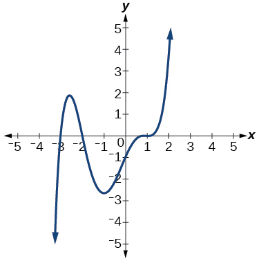
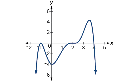
What can we conclude about the polynomial represented by the graph shown below based on its intercepts and turning points?

$CNX_Precalc_Figure_03_03_222.jpg$

A polynomial function

Answer

The end behavior indicates an odd-degree polynomial function (ends in opposite direction), with a negative leading coefficient (falls right). There are 3 $x$-intercepts each with odd multiplicity, and 2 turning points, so the degree is odd and at least 3.

Write a Formula for a Polynomial given its Graph

Now that we know how to find zeros of polynomial functions, we can use them to write formulas based on graphs. Because a polynomial function written in factored form will have an $x$-intercept where each factor is equal to zero, we can form a function that will pass through a set of $x$-intercepts by introducing a corresponding set of factors.

Note: Factored Form of Polynomials

If a polynomial of lowest degree $p$ has horizontal intercepts at $x=x_1,x_2,…,x_n$, then the polynomial can be written in the factored form: $f(x)=a(x−x_1)^(x−x_2)^⋯(x−x_n)^$ where the powers $p_i$ on each factor can be determined by the behavior of the graph at the corresponding intercept, and the stretch factor $a$ can be determined given a value of the function other than the $x$-intercept.

How to: Given a graph of a polynomial function, write a formula for the function.

Identify the $x$-intercepts of the graph to find the factors of the polynomial.
Examine the behavior of the graph at the $x$-intercepts to determine the multiplicity of each factor.
Find the polynomial of least degree containing all the factors found in the previous step.
Use any other point on the graph (the $y$-intercept may be easiest) to determine the stretch factor.

Example $\PageIndex$: Writing a Formula for a Polynomial Function from the Graph

Construct the factored form of a possible equation for each graph given below.

Solution

Looking at the graph of this function, as shown in Figure $\PageIndex$, it appears that there are $x$-intercepts at $x=−3,−2, \text< and >1$.

Each $x$-intercept corresponds to a zero of the polynomial function and each zero yields a factor, so we can now write the polynomial in factored form.

The stretch factor $a$ can be found by using another point on the graph, like the $y$-intercept, $(0,-6)$.

Solution

This graph has three $x$-intercepts: $x=−3,\;2,\text< and >5$. The $y$-intercept is located at $(0,2).$ At $x=−3$ and $ x=5$, the graph passes through the axis linearly, suggesting the corresponding factors of the polynomial will be linear. At $x=2$, the graph bounces at the intercept, suggesting the corresponding factor of the polynomial will be second degree (quadratic). Together, this gives us

To determine the stretch factor, we utilize another point on the graph. We will use the $y$-intercept $(0,–2)$, to solve for $a$.

The graphed polynomial appears to represent the function $f(x)=\dfrac(x+3)(x−2)^2(x−5)$.

Try It $\PageIndex$: Construct a formula for a polynomial given a graph

Given the graph shown in Figure $\PageIndex$, write a formula for the function shown.

$Graph of a negative even-degree polynomial with zeros at x=-1, 2, 4 and y=-4.$

Answer

Try It $\PageIndex$: Construct a formula for a polynomial given a description

Write a formula for a polynomial of degree 5, with zeros of multiplicity 2 at $x$ = 3 and $x$ = 1, a zero of multiplicity 1 at $x$ = -3, and vertical intercept at (0, 9)

Answer

$f(x) = \dfrac (x - 1)^2 (x - 3)^2 (x + 3)$

Key Concepts

Polynomial functions of degree 2 or more are smooth, continuous functions.
To find the zeros of a polynomial function, if it can be factored, factor the function and set each factor equal to zero.
Another way to find the $x$-intercepts of a polynomial function is to graph the function and identify the points at which the graph crosses the $x$-axis.
The multiplicity of a zero determines how the graph behaves at the $x$-intercepts.
The graph of a polynomial will cross the horizontal axis at a zero with odd multiplicity.
The graph of a polynomial will touch the horizontal axis at a zero with even multiplicity.
The end behavior of a polynomial function depends on the leading term.
The graph of a polynomial function changes direction at its turning points.
A polynomial function of degree $n$ has at most $n−1$ turning points.
To graph polynomial functions, find the zeros and their multiplicities, determine the end behavior, and ensure that the final graph has at most $n−1$ turning points.

Glossary

multiplicity
the number of times a given factor appears in the factored form of the equation of a polynomial; if a polynomial contains a factor of the form $(x−h)^p$, $x=h$ is a zero of multiplicity $p$.

Contributors

Jay Abramson (Arizona State University) with contributing authors. Textbook content produced by OpenStax College is licensed under a Creative Commons Attribution License 4.0 license. Download for free at https://openstax.org/details/books/precalculus.

3.4: Graphs of Polynomial Functions is shared under a CC BY license and was authored, remixed, and/or curated by LibreTexts.

Back to top
- 3.3e: Exercises - Polynomial End Behaviour
- 3.4e: Exercises - Polynomial Graphs

Was this article helpful?
Yes
No

3.4: Graphs of Polynomial Functions

Identify Zeros and Their Multiplicities from a Graph

Find Zeros and their Multiplicities from a Polynomial Equation

Graph Polynomial Functions

Turning Points

Write a Formula for a Polynomial given its Graph

Key Concepts

Glossary

Contributors

Recommended articles